Adaptable Dimension Embeddings: A Technical Guide for AI Engineers and Software Developers

Introduction: Why Dimension Size Matters in AI Systems

As a software engineer or ML practitioner building AI-powered applications, you've likely encountered the fundamental role of embeddings—numerical vector representations that encode semantic information about text, images, or other data types. These embeddings power everything from similarity search to classification and recommendation systems.

However, you've probably also faced a critical engineering challenge: embedding dimensions create unavoidable trade-offs in your AI systems:

1Higher dimensions → Better accuracy → Higher costs & slower performance
2Lower dimensions → Faster performance → Potentially worse accuracy

This technical dilemma traditionally forced engineers to choose a fixed dimension size and accept the associated limitations. Adaptive dimension embeddings, enabled by techniques like Matryoshka Representation Learning (MRL), provide a powerful solution that lets you dynamically adjust this trade-off based on your application's needs.

This guide will walk you through:

The technical foundations of adaptive dimension embeddings
How to implement and utilize them in production systems
Performance benchmarking and optimization techniques
Practical coding patterns for different use cases

Implementing Adaptable Dimension Embeddings in Your Code

Using OpenAI's Embedding Models with Variable Dimensions

OpenAI's `text-embedding-3-small` and `text-embedding-3-large` models directly support variable dimensions:

1from openai import OpenAI
2
3def get_embedding(text, dimension=1536):
4    """Get embedding with specified dimension"""
5    client = OpenAI()
6
7    response = client.embeddings.create(
8        model="text-embedding-3-small",
9        input=text,
10        dimensions=dimension  # Request specific dimension
11    )
12
13    return response.data[0].embedding
14
15# Example usage
16query_embedding_full = get_embedding("What is machine learning?", dimension=1536)
17query_embedding_reduced = get_embedding("What is machine learning?", dimension=256)
18
19# The reduced embedding retains most semantic information while being ~6x smaller
20

Using Open-Source MRL Models

Several open-source models also support variable dimensions, such as Nomic AI's models:

1from nomic import embed
2import numpy as np
3
4def get_nomic_embedding(texts, dimension=768):
5    """Get Nomic embeddings with specified dimension"""
6    output = embed.text(
7        texts=texts,
8        model='nomic-embed-text-v1.5',
9        task_type="search_document",
10        dimensionality=dimension  # Request specific dimension
11    )
12
13    return np.array(output['embeddings'])
14
15# Example usage
16docs = ["Machine learning is a field of AI", "Neural networks are popular in ML"]
17doc_embeddings = get_nomic_embedding(docs, dimension=256)
18

Implementation Tutorial: Building MRL From Scratch

Let's implement a complete MRL system using PyTorch. We'll build a text classification system using the 20 Newsgroups dataset that generates embeddings at multiple dimensions (32, 64, 128, 256, 512, 768).

Step 1: Setting Up the Environment

First, let's set up our imports and prepare the dataset:

1import numpy as np
2import matplotlib.pyplot as plt
3from sklearn.datasets import fetch_20newsgroups
4from sklearn.feature_extraction.text import TfidfVectorizer
5from sklearn.metrics import accuracy_score
6from sklearn.model_selection import train_test_split
7import time
8import torch
9import torch.nn as nn
10import torch.optim as optim
11from torch.utils.data import DataLoader, TensorDataset
12
13# Set random seeds for reproducibility
14np.random.seed(42)
15torch.manual_seed(42)
16
17# Load data
18categories = ['alt.atheism', 'comp.graphics', 'sci.med', 'soc.religion.christian']
19newsgroups = fetch_20newsgroups(subset='all', categories=categories,
20                               remove=('headers', 'footers', 'quotes'))
21X, y = newsgroups.data, newsgroups.target
22
23# Create train/test split
24X_train, X_test, y_train, y_test = train_test_split(X, y, test_size=0.2, random_state=42)
25
26# Create initial features using TF-IDF
27vectorizer = TfidfVectorizer(max_features=2000)
28X_train_tfidf = vectorizer.fit_transform(X_train)
29X_test_tfidf = vectorizer.transform(X_test)
30
31# Convert to PyTorch tensors
32X_train_tensor = torch.FloatTensor(X_train_tfidf.toarray())
33X_test_tensor = torch.FloatTensor(X_test_tfidf.toarray())
34y_train_tensor = torch.LongTensor(y_train)
35y_test_tensor = torch.LongTensor(y_test)
36

Step 2: Designing the MRL Encoder Architecture

Now, let's create the MRL encoder that produces hierarchically structured embeddings:

1class MRLEncoder(nn.Module):
2    def __init__(self, input_dim, max_dim=768):
3        super(MRLEncoder, self).__init__()
4        self.max_dim = max_dim
5
6        # Encoder network - this produces the full-dimensional embedding
7        self.encoder = nn.Sequential(
8            nn.Linear(input_dim, 1024),
9            nn.ReLU(),
10            nn.Linear(1024, max_dim)
11        )
12
13        # Projection layers for different dimensions
14        # These ensure the embeddings have the nested Matryoshka structure
15        self.projections = nn.ModuleDict()
16        self.dims = [32, 64, 128, 256, 512, max_dim]
17
18        for dim in self.dims:
19            self.projections[str(dim)] = nn.Linear(max_dim, dim, bias=False)
20
21        # Critical step: Initialize projections to ensure nested structure
22        # This makes smaller embeddings subsets of larger ones
23        self._initialize_nested_projections()
24
25    def _initialize_nested_projections(self):
26        """Initialize projection matrices to enforce nested structure"""
27        with torch.no_grad():
28            for i, dim1 in enumerate(self.dims[:-1]):
29                dim2 = self.dims[i+1]
30                # Initialize so that projection to dim1 is equivalent to:
31                # 1. Projecting to dim2
32                # 2. Then taking the first dim1 dimensions
33                self.projections[str(dim1)].weight.data = \
34                    self.projections[str(dim2)].weight.data[:dim1, :]
35
36    def forward(self, x, dim=None):
37        """
38        Forward pass that can output embeddings at any requested dimension
39
40        Args:
41            x: Input tensor
42            dim: Target dimension (if None, returns max dimension)
43
44        Returns:
45            Embedding tensor at requested dimension
46        """
47        # Get the full-dimensional embedding from the encoder
48        full_emb = self.encoder(x)
49
50        # If no dimension specified or max dimension requested, return full embedding
51        if dim is None or dim == self.max_dim:
52            if dim == self.max_dim and str(dim) in self.projections:
53                return self.projections[str(dim)](full_emb)
54            return full_emb
55
56        # Use the appropriate projection for the requested dimension
57        if str(dim) in self.projections:
58            return self.projections[str(dim)](full_emb)
59        else:
60            # For dimensions not explicitly defined, find the nearest smaller one
61            available_dims = sorted([int(d) for d in self.projections.keys()])
62            nearest = max([d for d in available_dims if d <= dim])
63            return self.projections[str(nearest)](full_emb)[:, :dim]
64

Step 3: Building the Classification Head

Next, we'll create a classifier that works with multiple embedding dimensions:

1class MRLClassifier(nn.Module):
2    def __init__(self, input_dim, num_classes, max_dim=768):
3        super(MRLClassifier, self).__init__()
4        self.encoder = MRLEncoder(input_dim, max_dim)
5
6        # Create separate classification heads for each dimension
7        # This is important for optimizing classification at each dimension level
8        self.dims = [32, 64, 128, 256, 512, max_dim]
9        self.classifiers = nn.ModuleDict()
10
11        for dim in self.dims:
12            self.classifiers[str(dim)] = nn.Linear(dim, num_classes)
13
14    def forward(self, x, dim=None):
15        """
16        Forward pass with dimension-specific classification
17
18        Args:
19            x: Input tensor
20            dim: Target dimension (if None, uses max dimension)
21
22        Returns:
23            Classification logits
24        """
25        # Get embeddings at the specified dimension
26        emb = self.encoder(x, dim)
27
28        # Default to max dimension if none specified
29        if dim is None:
30            dim = self.encoder.max_dim
31
32        # Use the appropriate classifier for this dimension
33        if str(dim) in self.classifiers:
34            return self.classifiers[str(dim)](emb)
35        else:
36            # For non-standard dimensions, use the nearest smaller classifier
37            available_dims = sorted([int(d) for d in self.classifiers.keys()])
38            nearest = max([d for d in available_dims if d <= dim])
39            return self.classifiers[str(nearest)](emb[:, :nearest])
40

Step 4: Implementing the Multi-Dimension Training Loop

This is where MRL differs significantly from standard training. We need to train across multiple dimensions simultaneously:

1# Initialize the model
2input_dim = X_train_tfidf.shape[1]  # TF-IDF feature dimension
3num_classes = len(np.unique(y))     # Number of classes in dataset
4model = MRLClassifier(input_dim, num_classes)
5
6# Training parameters
7batch_size = 64
8train_dataset = TensorDataset(X_train_tensor, y_train_tensor)
9train_loader = DataLoader(train_dataset, batch_size=batch_size, shuffle=True)
10criterion = nn.CrossEntropyLoss()
11optimizer = optim.Adam(model.parameters(), lr=0.001)
12
13# Training loop
14num_epochs = 5
15dims_to_train = [32, 64, 128, 256, 512, 768]  # Train all dimensions
16
17for epoch in range(num_epochs):
18    model.train()
19    total_loss = 0
20
21    for batch_X, batch_y in train_loader:
22        # Critical: Train each dimension in each batch
23        # This ensures all dimensions learn effectively
24        for dim in dims_to_train:
25            # Forward pass at this dimension
26            optimizer.zero_grad()
27            outputs = model(batch_X, dim)
28
29            # Calculate loss and backpropagate
30            loss = criterion(outputs, batch_y)
31            loss.backward()
32            optimizer.step()
33
34            total_loss += loss.item()
35
36    # Print progress
37    avg_loss = total_loss / (len(train_loader) * len(dims_to_train))
38    print(f"Epoch {epoch+1}/{num_epochs}, Avg Loss: {avg_loss:.4f}")
39

Step 5: Evaluation and Performance Analysis

Now let's evaluate our model across different dimensions to see the accuracy-efficiency tradeoff:

1# Evaluate performance at each dimension
2model.eval()
3results = []
4
5for dim in dims_to_train:
6    start_time = time.time()
7
8    with torch.no_grad():
9        outputs = model(X_test_tensor, dim)
10        _, predicted = torch.max(outputs, 1)
11
12    # Calculate inference time
13    inference_time = time.time() - start_time
14
15    # Calculate accuracy
16    accuracy = accuracy_score(y_test, predicted.numpy())
17
18    # Calculate storage requirements (in KB)
19    # Assuming 4 bytes per float (32-bit floating point)
20    storage_kb = (dim * 4) / 1024
21
22    # Store results
23    results.append({
24        'dimension': dim,
25        'accuracy': accuracy,
26        'inference_time': inference_time,
27        'storage_kb': storage_kb
28    })
29
30    print(f"Dimension: {dim}, Accuracy: {accuracy:.4f}, "
31          f"Inference Time: {inference_time:.4f}s, Storage: {storage_kb:.2f}KB")
32
33# Create a performance comparison table
34from tabulate import tabulate
35table_data = [[r['dimension'], f"{r['accuracy']:.4f}",
36               f"{r['inference_time']*1000:.2f}ms", f"{r['storage_kb']:.2f}KB"]
37              for r in results]
38headers = ["Dimension", "Accuracy", "Inference Time", "Storage"]
39print(tabulate(table_data, headers, tablefmt="grid"))
40

Step 6: Visualization and Analysis

Let's visualize our results to understand the performance-efficiency tradeoff:

1# Visualization of results
2plt.figure(figsize=(15, 5))
3
4# Plot accuracy vs dimension
5plt.subplot(1, 3, 1)
6plt.plot([r['dimension'] for r in results], [r['accuracy'] for r in results], 'o-')
7plt.xlabel('Embedding Dimension')
8plt.ylabel('Accuracy')
9plt.title('Accuracy vs Embedding Dimension')
10plt.grid(True)
11
12# Plot storage vs dimension
13plt.subplot(1, 3, 2)
14plt.plot([r['dimension'] for r in results], [r['storage_kb'] for r in results], 'o-')
15plt.xlabel('Embedding Dimension')
16plt.ylabel('Storage (KB)')
17plt.title('Storage Requirements vs Dimension')
18plt.grid(True)
19
20# Plot accuracy vs storage
21plt.subplot(1, 3, 3)
22plt.plot([r['storage_kb'] for r in results], [r['accuracy'] for r in results], 'o-')
23plt.xlabel('Storage (KB)')
24plt.ylabel('Accuracy')
25plt.title('Accuracy vs Storage Trade-off')
26plt.grid(True)
27
28plt.tight_layout()
29plt.savefig('mrl_performance_tradeoff.png')
30plt.show()
31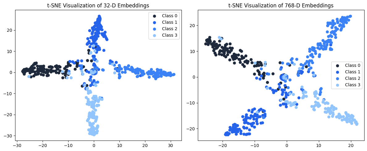

Step 7: Bonus - Visualizing Embedding Structure with t-SNE

To understand how well our embeddings preserve class information across dimensions:

1from sklearn.manifold import TSNE
2
3# Get embeddings at different dimensions
4all_embeddings = {}
5with torch.no_grad():
6    for dim in [32, 768]:  # Compare smallest and largest
7        embeddings = model.encoder(X_test_tensor, dim).numpy()
8        all_embeddings[dim] = embeddings
9
10# Apply t-SNE to reduce to 2D for visualization
11tsne_results = {}
12for dim, emb in all_embeddings.items():
13    # For speed, use a sample of the test set
14    sample_size = min(500, len(emb))
15    sample_indices = np.random.choice(len(emb), sample_size, replace=False)
16    sample_embeddings = emb[sample_indices]
17    sample_labels = y_test[sample_indices]
18
19    # Apply t-SNE
20    tsne = TSNE(n_components=2, random_state=42)
21    tsne_result = tsne.fit_transform(sample_embeddings)
22    tsne_results[dim] = (tsne_result, sample_labels)
23
24# Plot t-SNE visualizations
25plt.figure(figsize=(12, 5))
26for i, dim in enumerate([32, 768]):
27    plt.subplot(1, 2, i+1)
28    tsne_result, labels = tsne_results[dim]
29
30    # Plot each class with a different color
31    for class_idx in range(num_classes):
32        mask = labels == class_idx
33        plt.scatter(tsne_result[mask, 0], tsne_result[mask, 1],
34                   label=f'Class {class_idx}')
35
36    plt.title(f't-SNE Visualization of {dim}-D Embeddings')
37    plt.legend()
38
39plt.tight_layout()
40plt.savefig('mrl_tsne_visualization.png')
41plt.show()
42

Implementing Adaptive Retrieval for Optimized Search

One of the most powerful applications of adaptable dimension embeddings is a technique called "Adaptive Retrieval," which dramatically improves search performance.

The Two-Pass Approach

Adaptive Retrieval uses a two-stage process to balance speed and accuracy:

First pass: Use low-dimensional embeddings (e.g., 256d) to quickly find potential matches
Second pass: Re-rank the top candidates using high-dimensional embeddings (e.g., 1536d)

This approach can achieve up to 10-14x speed improvements with negligible accuracy loss.

Implementation Example

1def adaptive_retrieval(query, vector_db, embedding_model, low_dim=256, high_dim=1536):
2    """
3    Perform two-stage retrieval using adaptive dimensions
4
5    Args:
6        query: The search query text
7        vector_db: Vector database instance
8        embedding_model: Model that supports variable dimensions
9        low_dim: Dimension for initial fast search
10        high_dim: Dimension for accurate re-ranking
11
12    Returns:
13        List of ranked results
14    """
15    # Generate low-dimensional query embedding for fast initial search
16    query_embedding_low = embedding_model.embed(query, dimension=low_dim)
17
18    # First pass: Retrieve candidate set using fast low-dim search
19    # Typically retrieve more results than needed (e.g., 100-200)
20    candidates = vector_db.search(
21        vector=query_embedding_low,
22        dimension=low_dim,
23        limit=200
24    )
25
26    # Extract candidate IDs
27    candidate_ids = [item['id'] for item in candidates]
28
29    # Get high-dimensional embeddings for candidates
30    candidate_vectors = vector_db.get_vectors_by_ids(
31        ids=candidate_ids,
32        dimension=high_dim
33    )
34
35    # Generate high-dimensional query embedding for accurate scoring
36    query_embedding_high = embedding_model.embed(query, dimension=high_dim)
37
38    # Second pass: Re-rank candidates using high-dimensional similarity
39    results = []
40    for doc_id, vector in candidate_vectors.items():
41        # Calculate similarity (e.g., cosine similarity)
42        similarity = cosine_similarity(query_embedding_high, vector)
43        results.append({
44            'id': doc_id,
45            'score': similarity
46        })
47
48    # Sort by similarity score (descending)
49    results.sort(key=lambda x: x['score'], reverse=True)
50
51    # Return top results (e.g., top 10)
52    return results[:10]
53

Vector Database Considerations

Implementing adaptive retrieval requires a vector database that supports:

Indexing and searching at different dimensions: The database must efficiently search embeddings at the lower dimension
Efficient batch retrieval by ID: For quickly retrieving full-dimensional vectors of candidates
Optional but helpful - Hybrid indexes: Some databases support creating special indexes that store multiple dimension versions

Production Implementation Patterns

When deploying adaptable dimension embeddings in production, consider these architectural patterns:

1. Embedding Pipeline with Dimension Branching

1Input Text → Embedding Generation → Store Multiple Dimensions
2                                     ├→ Full Dim (DB #1)
3                                     ├→ Mid Dim (DB #2)
4                                     └→ Low Dim (DB #3)
5

2. Single Database with Multi-Dimensional Indexing

1Query → Low-Dim Search → Candidate Set → High-Dim Re-ranking → Results
2

3. Progressive Loading Pattern

1Initial Request → Low-Dim Results (fast) →
2    Background Load → Mid-Dim Results →
3        User Interaction → High-Dim Final Results
4

Conclusion: Best Practices for Engineers

As you implement adaptable dimension embeddings in your ML systems, keep these best practices in mind:

Benchmark extensively: Don't assume theoretical performance gains; measure the accuracy-speed-storage tradeoffs for your specific use case.
Start with the simplest approach: Begin with basic dimension truncation before implementing complex adaptive retrieval.
Monitor key metrics: Track embedding generation time, query latency, storage usage, and accuracy metrics across different dimensions.
Consider your infrastructure: Ensure your vector database supports efficient operations at different dimensions.
Build progressive systems: Design your architecture to start with fast, low-dimensional processing and progressively enhance with higher dimensions where needed.

Mastering adaptable dimension embeddings gives you a powerful tool for optimizing AI systems, allowing you to find the perfect balance between performance, cost, and accuracy for your specific application requirements.

By implementing the techniques in this guide, you'll be well-equipped to build more efficient and scalable AI systems that deliver better user experiences while controlling infrastructure costs.

---

Want to see practical implementations of these concepts? After reading this guide, check out our reference implementation on GitHub for complete code examples, benchmarking tools, and additional resources to help you implement adaptable dimension embeddings in your own projects.

---

Looking to level up your AI engineering skills? Join our community of engineers implementing cutting-edge techniques in production. Sign up for our newsletter for weekly technical deep dives and code examples.